CO Problems
We show the basic denotations of graphs. Let \(\mathcal{G} = (\mathcal{V}, \mathcal{E}, W)\) denote a weighted graph, where \(\mathcal{V}\) is the node set, \(\mathcal{E}\) is the edge set, \(|\mathcal{V}| = V\), \(|\mathcal{E}| = E\), and \(W : \mathcal{E} \rightarrow \mathbb{R}^+\) is the edge weight function, i.e., \(W_{u,v}\) is the weight of edge \((u,v) \in \mathcal{E}\). \(W_{u,v} > 0\) if \((u,v)\) is an edge and 0 otherwise. Let \(\delta^+(i)\) and \(\delta^-(i)\) denote the out-arcs and in-arcs of node \(i\).
Integer linear programming (ILP) is a standard formulation of combinatorial optimization problems. It has the canonical form:
where \(\mathbf{x}\) is a vector of \(n\) decision variables, \(\mathbf{c}\) is a vector of \(n\) coefficients for \(\mathbf{x}\) in the objective function, \(A \in \mathbb{R}^{m \times n}\) and \(\mathbf{b} \in \mathbb{R}^m\) together denote \(m\) linear constraints, and \(\mathbf{x} \in \mathbb{Z}^n\) implies that we are interested in integer solutions. Let \(\mathbf{x}^*\) denote the optimal solution and \(f^*\) denote the corresponding objective value. Only a few problems such as portfolio optimization are quadratic programming, which will be described later.
With respect to QUBO or Ising model, we consider a 1D Ising model with a ring structure and an external magnetic field \(h_i\). There are \(N\) nodes with \((N + 1) \equiv 1 \mod N\); a node \(i\) has a spin \(s_i \in \{+1, -1\}\) (where +1 for up and −1 for down). Two adjacent sites \(i\) and \(i + 1\) have an energy \(w_{i,i+1}\) or \(-w_{i,i+1}\) depending on whether they have the same or different directions, respectively.
The whole system will evolve into the ground state with the minimum Hamiltonian:
where \(\alpha\) is a weight, \(f_A\) is defined on each node’s effect on its own, and \(f_B\) is defined on each two adjacent nodes’ interactions. In fact, we generally use binary variables (0 or 1) to formulate the objective function, and \(s_i \in \{+1, -1\}\) can be replaced by
where \(x_i \in \{0, 1\}\).
Graph Maxcut
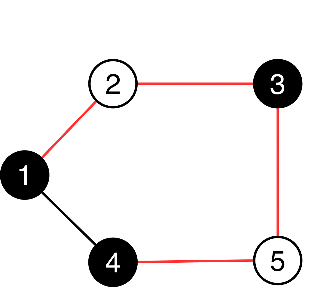
Figure 1: An example of graph maxcut.
The graph maxcut problem is defined as follows. Given a graph \(\mathcal{G} = (\mathcal{V}, \mathcal{E}, W)\), split \(\mathcal{V}\) into two subsets \(\mathcal{V}^+\) (with edge set \(\mathcal{E}^+\)) and \(\mathcal{V}^-\) (with edge set \(\mathcal{E}^-\)), and the cut set is \(\delta = \{(i, j) \mid i \in \mathcal{V}^+, j \in \mathcal{V}^-\}\). The goal is to maximize the cut value:
Where \(W_{ij}\) represents the importance (or cost) of edge \((i, j)\), and is usually predefined based on the graph structure.
1. ILP Formulation
Take Figure 1 for Example
s.t.
Each \(\mathbf{x}, \mathbf{y}\in \{0, 1\}\).
This ILP formulation ensures that \(\mathbf{y}_{ij} = 1\) if and only if nodes \(i\) and \(j\) belong to different subsets (i.e., edge \((i,j)\) is cut).
We provide general ILP formulation of graph maxcut
where \(x_i\) is a binary variable denoting if node \(i\) belongs to the selected subset; and \(y_{ij}\) is 1 if nodes \(i\) and \(j\) are in different subsets and 0 otherwise. The weight \(W_{ij}\) represents the importance (or cost) of edge \((i, j)\), and is usually predefined based on the graph structure.
2. QUBO Formulation
Take Figure 1 for example
For an illustrative example in the left graph of Figure 1, the edge set is:
\(E = \{(1,2), (1,4), (2,3), (2,4), (3,5)\}\)
and the weights are:
\(w_{12} = w_{14} = w_{23} = w_{24} = w_{35} = w_{45} = 1\).
The edge set of black nodes is \(\mathcal{E}^+ = \{(1, 4)\}\), and the edge set of white nodes is \(\mathcal{E}^- = \emptyset\).
The edges connecting the two subsets are:
\(\delta = \{(1,2), (2,3), (2,4), (3,5), (4,5)\}\).
The solution is \(x \in \{0,1\}^5\), and the Hamiltonian in Equation (3) becomes:
We provide general QUBO formulation of maxcut
Here, \(\sum_{(i,j)\in \mathcal{E}} W_{ij}\) is a constant. Let \(x_i = 1\) if node \(i\) belongs to \(V^+\), and 0 otherwise. The term \(1 - (2x_i - 1)(2x_j - 1)\) equals 1 if nodes \(i\) and \(j\) are in different subsets, and 0 otherwise.
3. RL Methods: Two Decision Patterns
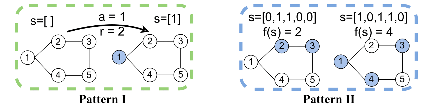
Figure 2: Two patterns for graph maxcut.
Sparse-rewards Pattern (I) Initial state is empty. RL agent selects node 1 with the highest Q-value. Reward is 2. New state becomes :math:[1].
Dense-rewards Pattern (II) Current state is :math:[2, 3], objective = 2. Agent adds node 1. New state is :math:[1, 3, 4]. Objective improves to 4.
Knapsack
We take knapsack as a second probelm.
Knapsack problem Given a set of items \(\mathcal{I}\), each item \(i\) with an integer weight \(W_i\) and a value \(\mu_i\), determine which items to include in the collection so that the total weight is less than or equal to a given limit \(U\) and the total value is maximized.
We assume there are 3 items. Their values are \([1, 1, 2]\), weights are \([1, 1, 1]\), and the total weight limit is \(2\).
1. ILP Formulation
ILP formulation for this example
We provide general ILP formulation of knapsack
where \(x_i\) is a binary variable (1 if item \(i\) is in the knapsack), \(\mu_i\) is its value, \(W_i\) is its weight, and \(U\) is the weight limit.
2. QUBO Formulation
For the same example:
We consider an item \(i\), and let \(x_i\) be a binary variable with 1 denoting it is in the knapsack and 0 otherwise. Let \(y_n\) for \(1 \leq n \leq U\) be a binary variable with 1 denoting the final weight of the knapsack is \(n\).
The QUBO formulation of Knapsack is:
Here, \(y_1, y_2\) are binary variables indicating whether total weight equals 1 or 2 respectively. \(\alpha \in (0,1)\) is a penalty parameter.
We provide general QUBO formulation of knapsack
where \(y_n \in \{0,1\}\) denotes whether the final weight equals \(n\), and \(x_i\) is whether item \(i\) is in the knapsack.
3. Two Patterns of RL Methds
For the same 3-item knapsack problem
Pattern I The initial state is empty. Then we select item 2 and add it to the state, i.e., the new state is :math:[2]. The reward is 1.
Pattern II The current state is :math:[0, 1, 0], and the objective value is 1. The new state is :math:[0, 1, 1], and the objective value is 3.