Quickstart

The following processes show how to run the algorithms.

Read Data

There are two types of datasets used:

• Gset: Provided by Stanford University, stored in the data/ folder. The number of nodes ranges from 800 to 10,000.

• Syn: Synthetic data. Number of nodes ranges from 100 to 1000 across three distributions: Barabasi–Albert (BA), Erdos–Renyi (ER), and Powerlaw (PL). Each distribution has 10 graph instances.

Example: gset_14.txt (an undirected graph with 800 nodes and 4694 edges):

800 4694          # nodes = 800, edges = 4694
1 7 1             # node 1 connects with node 7, weight = 1
1 10 1            # node 1 connects with node 10, weight = 1
1 12 1            # node 1 connects with node 12, weight = 1

Store Solution

The solution will be stored in the folder result.

Take graph maxcut as an example. The result includes the objective value, number of nodes, algorithm name, and the solution.

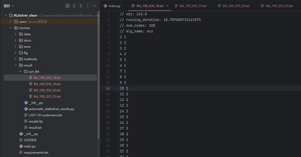
Example result for data/syn_BA/BA_100_ID0.txt stored in result/syn_BA/BA_100_ID0.txt:

// obj: 273.0        # objective value
// running_duration: 71.9577648639679
// num_nodes: 100
// alg_name: greedy

1 1   # node 1 in set 1
2 2   # node 2 in set 2
3 2   # node 3 in set 2
4 2   # node 4 in set 2
5 2   # node 5 in set 2
...

Distribution-wise

1. Select problem

In config.py, we select a CO problem:

PROBLEM = Problem.maxcut  # We can select a problem such as maxcut.

2. Training

Take S2V-DQN as an example, as proposed by Dai et al. (2017) in Learning Combinatorial Optimization Algorithms over Graphs.

During training, the reinforcement learning agent explores how graph structures relate to optimal (or near-optimal) solutions such as maximum cuts. Through repeated trial and reward, it gradually learns a general strategy that can be applied to new, unseen graphs with similar characteristics.

2.1. Set basic config:

Edit rlsolver/methods/eco_s2v/config.py.

ALG = Alg.s2v                                   # select s2v as the RL method
GRAPH_TYPE = GraphType.BA                       # use BA (Barabási–Albert) graph distribution
NUM_TRAIN_NODES = 20                            # each training graph has 20 nodes
TRAIN_INFERENCE = 0                             # 0 = train mode; 1 = inference mode

2.2. Run training:

Run rlsolver/methods/eco_s2v/main.py.

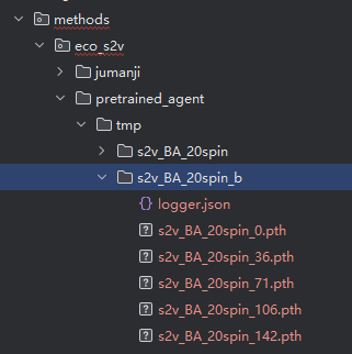
python rlsolver/methods/eco_s2v/main.py

This will generate a folder: rlsolver/methods/eco_s2v/pretrained_agent/tmp/s2v_BA_20spin_b/

Inside this folder, multiple .pth model snapshots will be saved over time.

2.3. Select the best model from this folder:

Edit rlsolver/methods/eco_s2v/config.py.

Find the line:

NEURAL_NETWORK_SUBFOLDER = "s2v_BA_20spin_s"

To select a different model folder, set the param NEURAL_NETWORK_SUBFOLDER using the name of the desired folder. For example:

NEURAL_NETWORK_SUBFOLDER = "s2v_BA_20spin_b"

Then run: rlsolver/methods/eco_s2v/train_and_inference/select_best_neural_network.py.

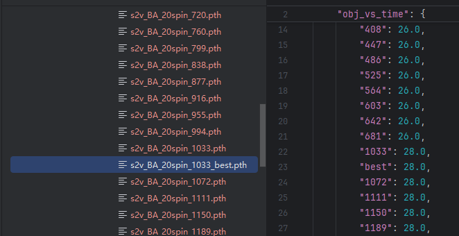
python rlsolver/methods/eco_s2v/train_and_inference/select_best_neural_network.py

It will generate a file like: s2v_BA_20spin_1033_best.pth

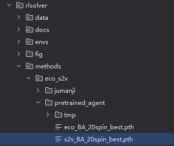
2.4. Rename and move the best model:

s2v_BA_20spin_best.pth → rlsolver/methods/eco_s2v/pretrained_agent/

3. Testing

Now that training is complete and the best model has been selected and moved, we proceed to the testing phase. The following steps configure and run inference using the trained model on graphs of various sizes.

3.1. Switch to inference mode:

Edit rlsolver/methods/eco_s2v/config.py.

TRAIN_INFERENCE = 1                                              # 1 = inference mode
NUM_TRAINED_NODES_IN_INFERENCE = 20              # model was trained on 20-node graphs
NUM_INFERENCE_NODES = [20, 100, 200, 400, 800]   # test on graphs of various sizes

Although the model was trained only on 20-node graphs, it can be applied to larger graphs. Ensure that all test graphs have node counts ≥ 20.

3.2. Run inference:

Run rlsolver/methods/eco_s2v/main.py.

This step uses the selected best model to run inference over all test instances.

The result files will be saved in: rlsolver/result/syn_BA/

Each result file includes:

• obj: best objective value (maximum cut size)

• running_duration: solving time in seconds

• num_nodes: number of nodes in the graph

• alg_name: algorithm used (e.g., s2v)

• node assignments: each node’s group (1 or 2)

Example output:

This completes the full pipeline: Training → Model Selection → Inference for the s2v method on synthetic BA graphs.

Instance-wise

1. Select problem

In rlsolver/methods/config.py, we select a CO problem:

PROBLEM = Problem.maxcut

2. Select dataset(s)

In rlsolver/methods/config.py, we select dataset(s):

DIRECTORY_DATA = "../data/syn_BA"  # the directory of datasets
PREFIXES = ["BA_100_ID0"]             # select the BA graphs with 100 nodes

3. Run method

Run method in command line:

python methods/greedy.py                  # run greedy
python methods/gurobipy.py                # run gurobi
python methods/simulated_annealing.py     # run simulated annealing
python methods/mcpg.py                    # run MCPG
python methods/iSCO/main.py               # run iSCO

References

• Dai, H., Khalil, E. B., Zhang, Y., Dilkina, B., & Song, L. (2017). Learning Combinatorial Optimization Algorithms over Graphs. arXiv preprint arXiv:1704.01665.