Conventional Methods
Below is a brief description of each classical method implemented in RLSolver.
Gurobi
Gurobi Optimizer is a highly optimized commercial solver for linear, integer, and quadratic programs. For the MaxCut problem, RLSolver uses the Quadratic Unconstrained Binary Optimization (QUBO) formulation rather than the Integer Linear Programming (ILP) formulation, because QUBO typically yields higher solution quality and faster convergence; hence, Gurobi is set to solve the QUBO by default. It combines branch-and-bound, cutting planes, presolve reductions, and primal heuristics to efficiently navigate the solution tree and converge on an optimal (or provably near-optimal) solution.
Greedy
Greedy Heuristic is a fast, myopic heuristic that builds a solution one step at a time by always selecting the locally best choice. Although it lacks global optimality guarantees, its simplicity makes it a strong baseline and a useful warm-start for other methods.
Instance-wise Execution Guide
Although not an RL method, the greedy baseline provides a simple, interpretable benchmark to compare solution quality.
Set problem and dataset
In
rlsolver/methods/config.py, set the following:PROBLEM = Problem.maxcut DIRECTORY_DATA = "../data/gset" PREFIXES = ["gset_22"]
This will run the greedy algorithm on the Gset instance
gset_22.txt.Run Greedy
Use the following command to execute the baseline algorithm:
python rlsolver/methods/greedy.pyThis script runs greedy_maxcut() using the specified file(s) under data/gset/.
Result Output
After running the greedy algorithm, the results will be saved to:
rlsolver/result/syn_BA/
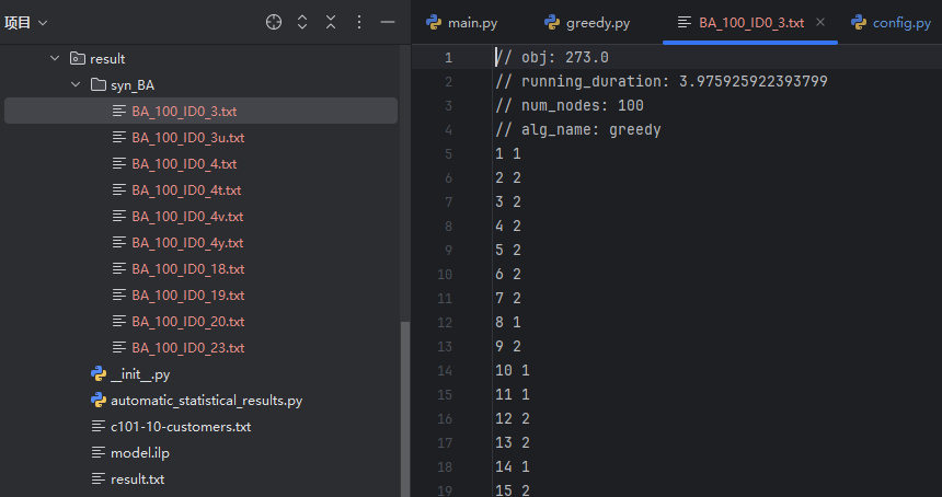
Each result file corresponds to one test instance and contains:
obj: Final objective value (e.g., total cut size for MaxCut).running_duration: Time taken by the algorithm in seconds.num_nodes: Number of nodes in the graph instance.alg_name: The algorithm used to generate the solution (e.g., greedy).Each following line: node ID and its assigned label (partition). For MaxCut, labels represent two sets in the cut.
The file is automatically generated and named based on the instance prefix and a unique suffix, such as:
BA_100_ID0_3.txt
SDP
Semidefinite Programming (SDP) approach lifts the original combinatorial problem into a higher-dimensional matrix space, turning it into a convex SDP. Solving the SDP yields a bound on the optimum; randomized rounding of the matrix solution then produces a high-quality feasible solution to the original problem.
SA
Inspired by the physical process of slow cooling in metallurgy, Simulated Annealing (SA) explores the solution space by occasionally accepting worse moves. The probability of accepting uphill (worsening) moves decreases over time (“temperature” schedule), allowing escape from local minima and gradual convergence.
GA
Genetic Algorithm (GA) maintains a population of candidate solutions (chromosomes). Each generation applies selection (keeping the fittest), crossover (recombining parts of two parents), and mutation (random small changes) to evolve toward better solutions over many iterations.